How to Alternate Row Colors in Google Sheets
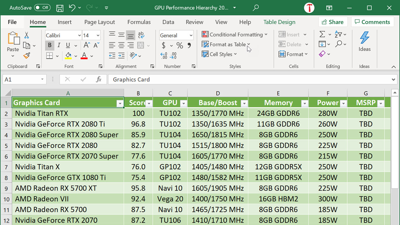
Shading cells in Excel or Google Sheets is a great way to format and organize your data and make your tables easier to read and present. You can easily apply alternate shading or color banding to rows or columns by using Excel's style tools or Sheets' formatting menu. There are multiple built-in templates readily available on both applications for you to choose from. But of course, if none of these options suit your preference or purpose, you can customize your worksheet by creating your own table style or by using conditional formatting.
How To Shade Alternate Rows in Excel using Format as Table
1. Select the cell range to format.
a. To format your entire worksheet, click the Select All section. This is the triangle icon located at the top left corner of the sheet before the first column.

b. To format an existing table, select all the cells in that table.
c. To format a subset of your worksheet, select the specific rows and columns you want to configure.
2. Choose the table style. On the Home tab, under the Styles group, click Format as Table and select a table style you prefer within the numerous templates provided in Excel. There are three template types: Light, Medium, and Dark. You can also create your own table style from this menu.
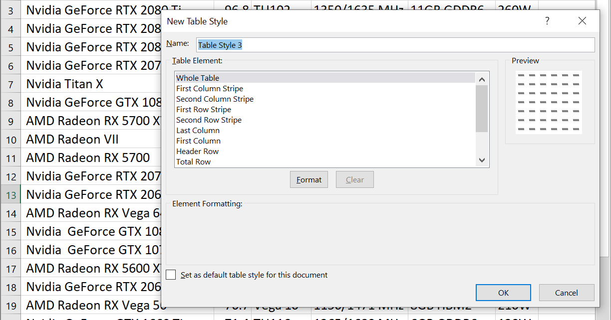
3. Click OK when done.
If you want to keep the alternate shading but don't need all the table functionalities such as sorting and filters, you can convert the excel table to a normal range. You can do this in two ways:
a. Click the Design tab under Table Tools. Click Convert to Range and click Yes when the confirmation notification pops up.
b. Select the table cells you want to convert, then right-click. Select Table from the menu and click Convert to Range.
How To Shade Alternate Rows in Excel using Conditional Formatting
1. Select the cell range to format. (Same rules as above apply.)
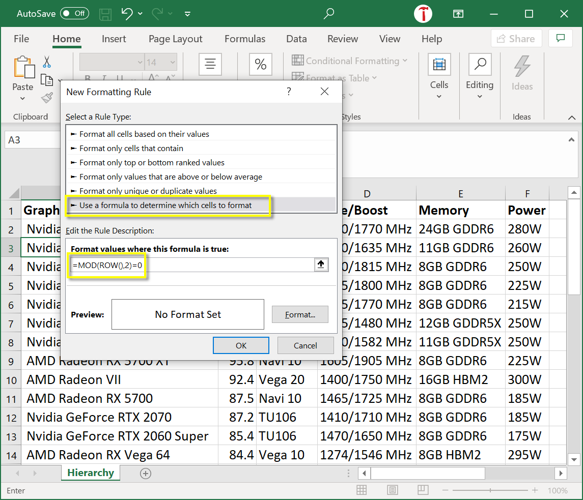
2. Navigate to the New Rules menu. On the Home tab, under the Styles group, click Conditional Formatting and select New Rule from the menu.
3. Select Rule Type. From the list of rule types, select Use a formula to determine which cells to format. Then type =MOD(ROW(),2)=0 command in the Rule Description field. (To shade alternate columns, type =MOD(COLUMN(),2)=0.)
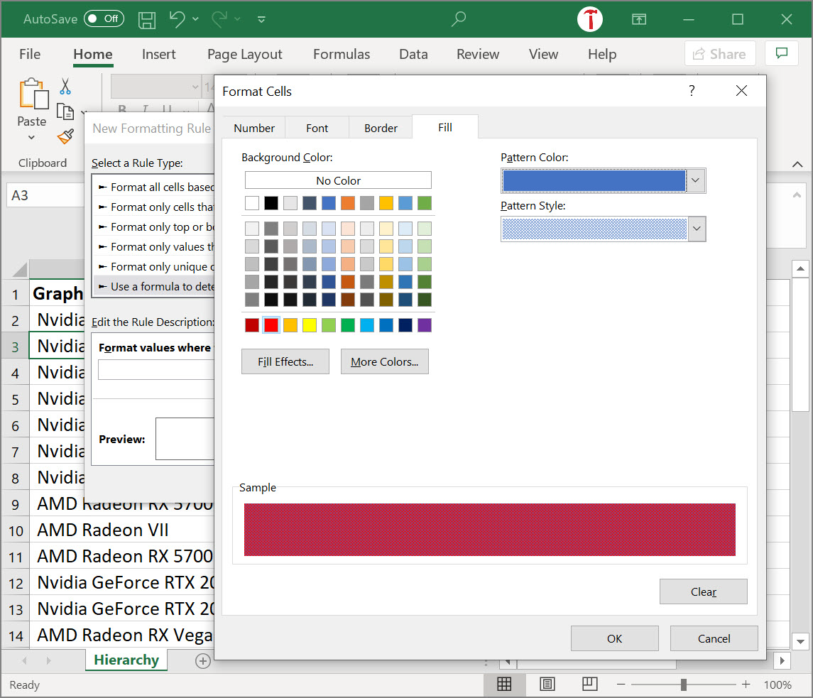
4. Choose a cell color. To do this, click Format, navigate to. the Fill tab and select a Background Color, a Pattern Color and even a Pattern Style. Click OK when done.
5. Check the preview box to make sure your selections were applied. Click OK. And you're done.
You can always go to the Manage Rules tool under Conditional Formatting if you want to delete or make changes to an existing rule.
How to Shade Alternate Rows in Google Sheets
1. Click Alternating Colours on the Format tab. A menu will pop up on the right side of your screen.
2. Set the range of cells to format.
3. Choose a style. You can use one of the default styles or customize to your own preference.

You can click Remove alternating colours easily if you change your mind.
How to Alternate Row Colors in Google Sheets
Source: https://www.tomshardware.com/how-to/shade-every-other-row-excel-google-sheets